SMC Case Studies
- Anova
- Firewire Case-Study
- Bluetooth Case-Study
- Train Gate Case-Study
- LMAC Case-Study
- LMAC 10-node Case-Study
- Duration Probabilistic Automata
- Distributed SMC
- Comparison with PVesta
- Control-SMC
Firewire Case-Study
We consider the IEEE 1394 High Performance Serial Bus (“FireWire” for short) that is used to transport video and audio signals on a network of multimedia devices. The protocol has two modes, one fast and one slow mode for the nodes. The model defines weights to enter these modes.
This is a leader election protocol that we model with two nodes. We
compute the probability for node 1 to become the root (or leader)
within different time bounds.
We use variable s to denote the state of a node. At
initialization, every node is in the contention state
s=0. After a sequence of steps, a node will enter the root
state s=7 and the other node will enter the child state
s=8.
The query formula is
Pr[time <= 1500] (<> node1.s==7 && node2.s==8)
We are also interested in checking whether there is a difference between the probability that a fast node becomes the root or the child and the probability that a slow node does. We use a probability comparison property for this purpose.
The results in the plot composer of Figure (a) show that the probability to elect node 1 as the root increases with the time bound. This probability density diagram shows that in most cases, node 1 may become the root after around 200 ms. UPPAAL confirms that the fastest possible to reach this state is 164 ms (with a standard reachability property). The result in Figure (b) shows that at the beginning the probabilities are indistinguishable, then the fast node has higher probability to become a root or a child, and at the end the probabilities become very close again.
We are also interested in checking whether there is a difference between the probability that a fast node becomes the root or the child and the probability that a slow node does. To model the two different modes of the nodes, we define two const array:
const int FAST[2]={80,80};

const int SLOW[2]={20,20};
These array are used as the probability weights in the probabilistic transitions. We can change the value of these array to make the two nodes different, for example:
const int FAST[2]={80,20};

const int SLOW[2]={20,80};
Now the node 1 will have the 80% probability to enter the fast mode while node 2 only 20% probability.
We use a probability comparison property for this purpose. The query
formula is
Pr[time <= 1500] (<> node1.s == 7 || node1.s == 8 )
>= Pr[time <= 1500] (<> node2.s == 7 || node2.s == 8
)
The result shows that at first, the two probability are indifferent
(both are 0), and then after about 200 time units, the node 1 has
higher probability to be a root or a child. Finally, the probability
becomes the same again (both are nearly 100%) after about 600 time
units.
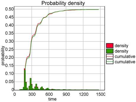 |
| (a) Probability to elect node 1. |
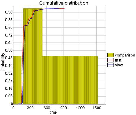 |
| (b) Probability comparison. |
Bluetooth Case-Study
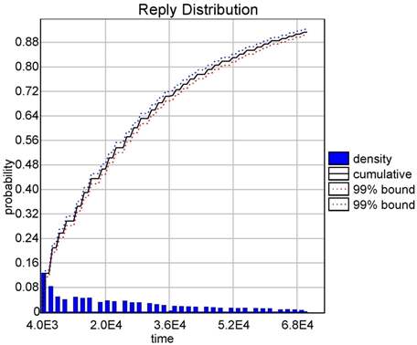
Bluetooth is a wireless telecommunication protocol using frequency-hopping to cope with interference between the devices in the network. A device can be in a scan state where it replies to a request after two time slots (a slot is 0.3125 ms) and goes to a reply state where it waits for a random amount of time before coming back to the scan state. When a device stays in the scan state, it can also enter the sleeping state (2012 time slots) to save energy. We model energy consumption with a clock (called energy) for which we change the rate depending on these states.
We check the following properties:
-
We evaluate the probability of replying within 70000 time units:
Pr[time <= 70000](<> receiver1.Reply)
The result is between [0.866977,0 966977]. -
We evaluate the probability of letting time pass 70000 time units with a limited energy budget:
Pr[energy <= 4000](<> time>=70000)
The result is between [0.949153,1].
In both cases the tool is able to compute a distribution of the probability over the bound given in argument. Figure (a) shows the cumulative probability of successfully communicating as a function of time. Figure (b) shows that it costs at least 2,400 energy units. The plot shows how bluetooth consumes energy.
This model is based on this
case-study
done with PRISM.
Model file.
Query file.
 |
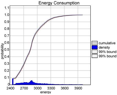 |
| (a) Probability to reply. | (b) Energy consumption. |
Train Gate Case-Study
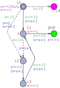
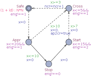
We consider our train-gate example (present in the demo directory of the distribution of UPPAAL and our tutorial), where N trains want to cross a one-track bridge. We extend the original model by specifying an arrival rate for Train i being (i+1)/N.
Trains are then approaching, but they can be stopped before some time threshold. When a train is stopped, it can start again. Eventually trains cross the bridge and go back to their safe state. The template of these trains is given in Figure (a). Our model captures the natual behaviour of arrivals with some exponential rate and random delays chosen with uniform distributions in states labelled with invariants.
The tool is used to estimate the probability that Train 0 and Train 5 will cross the bridge in less than 100 units of time. Given a confidence level of 0.05 the confidence intervals returned are [0.541,0.641] and [0.944,1]. The tool computes for each time bound T the frequency count of runs of length T for which the property holds. Figure (b) shows a superposition of both distributions obtained directly with our tool that provides a plot composer for this purpose.
The distribution for Train 5 is the one with higher probability at the beginning, which confirms that this train is indeed the faster one. An interesting point is to note the valleys in the probability densities that correspond to other trains conflicting for crossing the bridge. They are particularly visible for train 0. The number of valleys corresponds to the number of trains. This is clearly not a trivial distribution (not even unimodal) that we could not have guessed manually even from such a simple model. In addition, we use the qualitative check to cheaply refine the result to [0.541,0.59] and [0.97,1].
We then compare the probability for Train 0 to cross when all other trains are stopped with the same probability for Train 5. In the first plot (Figure (c) top), we check the same property with 100 different time bounds from 10 to 1000 in steps of 10 and we plot the number of runs for each check. These experiments only check for the specified bound, they are not parameterized. In the second plot, we use our parametric extension with a granularity of 10 time units. We configured the thresholds u0 and u1 to differentiate the comparisons at u0=1-ε and u1=1+ε with ε=0.1,0.05,0.01 as shown on the figure. In addition, we use a larger time bound to visualize the behaviours after 600 that are interesting for our checker. In the first plot of Figure (c), we show for each time bound the average of runs needed by the comparison algorithm repeated 30 times for different values of ε. In the bottom plot, we first superpose the cumulative probability for both trains (curves Train 0 and Train 5) that we obtain by applying our quantitative algorithm to evaluate probabilities for each time bound in the sampling. Interestingly, before that point, train 5 is better and later train 0 is better. Second, we compare these probabilities by using the comparison algorithm (curves 0.1 0.05 0.01). This algorithm can retrieve 3 values: 0 if Train 0 wins, 1 if Train 5 wins and 0.5 otherwise. We report for each time bound and each value of ε the average of these values for 30 executions of the algorithm.
In addition, to evaluate the efficiency of computing all results at once to obtain these curves, we measure the accumulated time to check all the 100 properties for the first plot (sequential check), and the time to obtain all the results at once (parallel check). The results are shown in Table (d). The experiments are done on a Pentium D at 2.4GHz and consume very little memory. The parallel check is about 10 times faster. In fact it is limited by the highest number of runs required as shown by the second peak in Figure (c). The expensive part is to generate the runs so reusing them is important. Note that at the beginning and at the end, our algorithm aborts the comparison of the curves, which is visible as the number of runs is sharply cut.
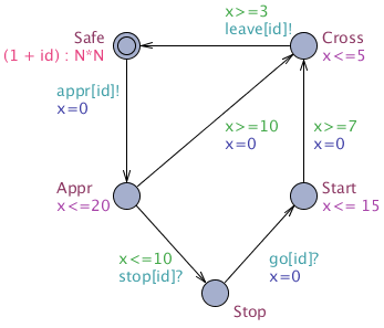 | ||||||||||||
| (a) Template of a train. | ||||||||||||
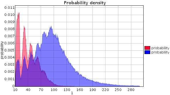 | ||||||||||||
(b) Probability density distributions for
<>(T≤t) Train(0).Cross
and
<>(T≤t) Train(5).Cross. | ||||||||||||
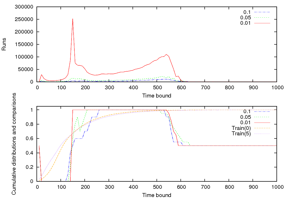 | ||||||||||||
| (c) Comparing train 0 and train 5. | ||||||||||||
| ||||||||||||
| (d) Sequential and parallel check comparison. |
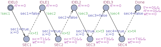
LMAC Case-Study
The Lightweight Media Access Control (LMAC) protocol is used in sensor
networks to schedule communication between nodes. This protocol is
targeted for distributed self-configuration, collision avoidance and
energy efficiency. In this study we reproduce the improved
UPPAAL model from
FHM2007
without verification
optimizations, parameterize with network topology (ring and chain),
add probabilistic weights (exponential and uniform) over discrete delay
decisions, and examine statistical properties which were not possible
to check before.
We examine four node network in a chain and a ring topologies as both topologies were identified in FHM2007 as problematic by having perpetual collisions, and two probabilistic weight distributions over choice of amount of frames to be waited: uniform (1,1,1,1) and exponential (4, 2, 1, 1).
The design of LMAC model in FHM2007 seems to favor the exponential
distribution as the node is making a binary decision after each
frame. Based on
Hoesel,
one of the LMAC implementations used 0.21mJ, 0.22mJ and 0.02mJ of
energy for transmitting, receiving and listening for messages
respectively. Since the model assumes fixed duration of each
operation, our node model consumes 21, 22, 2 and 1 power units per
time unit when a node is sending, receiving, listening for messages or
being idle respectively. The aggregate energy is computed by using a
global invariant energy’==sum(i: nodeid_t) power[i].
We use the following properties to examine the probabilistic properties of the model:
Pr[time <= 160] (<> exists(i:nodeid_t) Node(i).detected>=0)
Probability of collision.Pr[collisions <= 50000] (<> time>=1000)
Probability of collision count.Pr[energy <= 50000] (<> time>=1000)
Probability of energy consumption after 1000 time units.Pr[time <= 70] (<> col_count[1]>0) >= Pr[time <= 70] (<> col_count[2]>0)
Collision probability comparison of two networks.Pr[energy1 <= 10000] (<> time>=1000) >= Pr[energy2 <= 10000] (<> time>=1000)
Energy probability comparison of two networks.
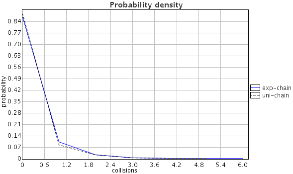
The results show that collisions persist but have rather low probability and there are some differences depending on the probabilistic weights. Figure (a) shows that collisions may happen in all cases and the probability of collision is higher with exponential decision weights than uniform decision weights, but seems independent of topology (ring or chain). The probability of collision stays stable after 61 time units, despite longer simulations, which means that the network may stay collision free if the first collisions are avoided. We also applied the method for parameterized probability comparision for the collision probability. The results are that up to 14 time units the probabilities are the same and later exponential weights have higher collision probability than uniform, but the results were inconclusive when comparing different topologies.
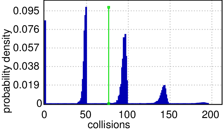
The probable collision count in the chain topology is shown in
Figure (b) where the case with 0 collisions has a
probability of 87.06% and 89.21% when using exponential and uniform
weights respectively. The maximum number of probable collisions are 7
for both weight distributions despite very long runs, which means
that the network eventually recovers from collisions.
The probable collision count in the ring topology (not shown) shows that there is no upper bound of collision count as the collisions add up, but there is still fixed probability peak at 0 collisions (87.06% and 88.39% using uniform and exponential weights resp.) with a short tail up to 7 collisions (like in Figure (b)), long interval of 0 probability and then small probability bump (0.35% in total) at large number of collisions. Thus the probability of perpetual collisions is tiny.
Figure (c) shows the energy consumption probability density: using uniform and exponential weights in a chain and a ring topologies. Ring topologies use more power (possibly due to collisions), and uniform weights use slightly less energy than exponential weights in these particular topologies.
We provided probabilistic evidence that sensor network in a ring and a chain topology may suffer perpetual collisions with probabilities slightly higher than 10%, but it is able to recover in a chain topology in a sense that there is rapidly decreasing probability of staying in a perpetual collision. There is some evidence that uniform weights in choosing delay might fair better.Model with probabilistic weights
model/query files.
Added collision counts and energy
model/query files.
Two network comparison
model/query files.
| Collision probability distribution and density using exponential and uniform weights in chain and ring topologies: (a) over time, (b) over collision count. |
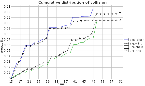 |
| (a) |
 |
| (b) |
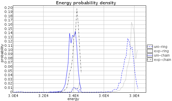 |
| (c) Network energy consumption. |
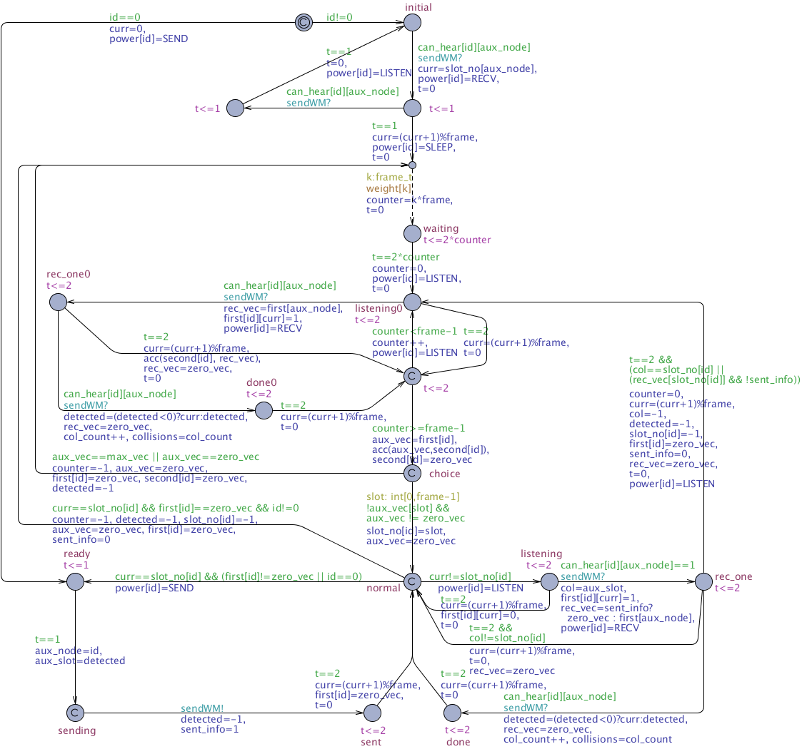 |
| (d) Model of a node. |
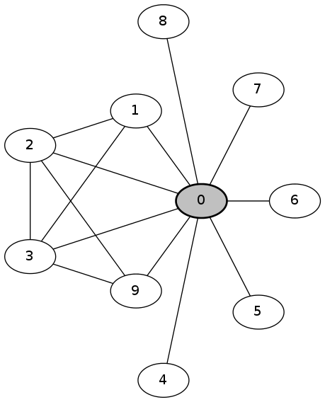
LMAC 10-node Case-Study
Larger sensor networks than five nodes are hardly verifiable by classical Uppaal, moreover the infinite loops of reoccurring collisions are not quantified probabilistically, hence one cannot assess the criticality of the issue. In this part we examine how SMC can be applied for larger networks and detect perpetual collisions using probabilistic means. The idea is that in cases with reoccurring collisions, the number of collisions diverge together with time.
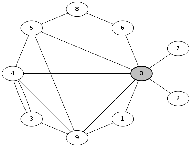
First, we sift through 10000 random topologies and find cases where the probability of hitting large number of collisions is high. Figure(a) shows the five topologies with highest probability Pr[<=2000](<> collisions>42). The verification takes about 6h 30min on a 32 core cluster. We can improve the topology search by heuristic construction of the connectivity graph, which yields 5120 non-isomorphic topologies. The computation on the same cluster took 3h 30min and the worst cases are displayed in the second row of Figure(b). The heuristic approach has clear advantages in performance, but does not guarantee the exhaustiveness.
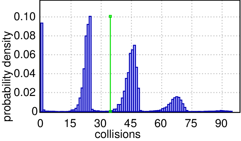
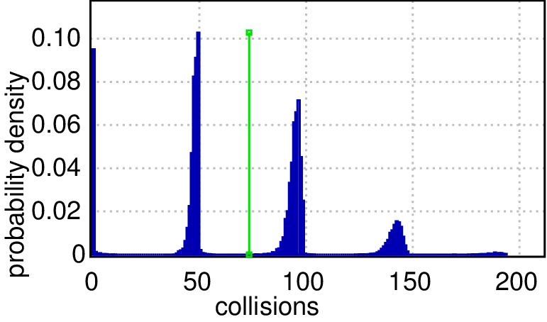
Second, we inspect the two worst cases in detail by computing the distribution of probable collision counts within 1000 and 2000 time units respectively. The queries are: Pr[collisions<=2000](<> time>=1000) and Pr[collisions<=2000](<> time>=2000) and the results are shown in Figures(c) and (d) respectively. In a chain and a ring topologies, mostly there are no collisions (>90% probability of zero collisions), but it is the other way around in our worst cases (>90% probability that there are many collisions). After a twice as long period of time, the plots show that the collision count distributions have the same shape, but the likely counts are twice as large (probability peaks shifted to the right), which imply that collisions keep happening perpetually and none of them disappeared in the longer run (even the absolute probability heights are preserved). The plots can be rendered with high precision, e.g. a cluster with 128 cores can generate 19 millions runs in 30 minutes, which are necessary for ±0.0005 precision and 99.98 confidence.
We have shown how perpetual collisions can be detected in LMAC network topologies with unprecedented size and estimate the likelihood of the undesired behavior.
Models: lmac-bubble.xml, lmac-star.xml.
Queries: lmac.q.
 |
 |
 |
| 0.63 | 0.63 | 0.62 |
|---|---|---|
| (a) Random topologies with large number of collisions. | ||
 |
 |
 |
| 0.92 | 0.91 | 0.90 |
|---|---|---|
| (b) Heuristically generated topologies with large number of collisions. | ||
 |
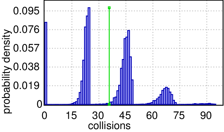 |
| (c) Probable collision counts within 1000 time units. | |
 |
 |
| (d) Probability density of a collision over time. | |
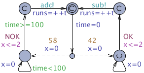
Duration Probabilistic Automata
Duration Probabilistic Automata MLK10 (DPA) are used for modelling jobshop problems. A DPA consists of several Simple DPAs (SDPA). An SDPA is a processing unit, a clock and a list of tasks to process sequentially. Each task has an associated duration interval, from which its duration is chosen (uniformly). Resources are used to model conflicts - we allow different resource types and different quantities of each type. A fixed priority scheduler is used to solve conflicts.
DPA can be encoded in our tool (with a continuous or discrete time semantic) or in PRISM (discrete semantic), see PV11. The performance of the translations have been tested on several case studies, see Table (a) and (b). In the verification column, UPPAAL uses our sequential hypothesis testing whereas PRISM uses its probabilistic model checking algorithm BK08. In the approximation column, both UPPAAL and PRISM use a quantitative check (evaluation of probability within some interval and with some confidence), but UPPAAL is faster thanks to its optimized implementation. Regarding UPPAAL, the error bounds used are α=β=0.05. In the hypothesis test, the indifference region size is 0.01, while we have ε=0.05 for the quantitative approach. The results show that the discrete encoding for UPPAAL is faster than PRISM.
In the first test, we create a DPA with n SDPAs, k tasks per SDPA and no resources. The duration interval of each task is changed and the time spend verifying is measured. In the second test, we choose n, k and let there be m resource types. We let a random generator decide the resource usage and duration interval. The query for the approximation test is: “With what probability do all SDPA end within t time units?”. In the verification test, we ask the query: “Do all SDPA end within t time units with probability greater than 40%?”. The value of t varies for each model; it was computed by simulating the system 369 times and represent the value for which at least 60% of the runs reached the final state.
In PRISM, integer and boolean variables are used to encode the current tasks and resources. PRISM only supports the discrete time model. In UPPAAL, a chain of waiting and task locations is created for each SDPA. Guards and invariants are used to encode the duration of the task, and an array of integers contains the available resources. The scheduler is encoded as a seperate template. For UPPAAL, both a discrete and continuous time version have been implemented.
Those experiments show that our tool is capable of handling models that are beyond the scope of the state-of-the art model checker for stochastic systems.
| ||||||||||||||||||||||||||||||||||||||||||||||||||||||||||||||||||||||||||||||||||||||||||||||||||||||||||||||||||||||||||||||||||||||||||||||||||||||||||||||||||||||||||||||||||||||
| (a) Tool performance comparison. | ||||||||||||||||||||||||||||||||||||||||||||||||||||||||||||||||||||||||||||||||||||||||||||||||||||||||||||||||||||||||||||||||||||||||||||||||||||||||||||||||||||||||||||||||||||||
| ||||||||||||||||||||||||||||||||||||||||||||||||||||||||||||||||||||||||||||||||||||||||||||||||||||||||||||||||||||||||||||||||||||||||||||||||||||||||||||||||||||||||||||||||||||||
| (b) Comparison with various durations. |
Distributed SMC
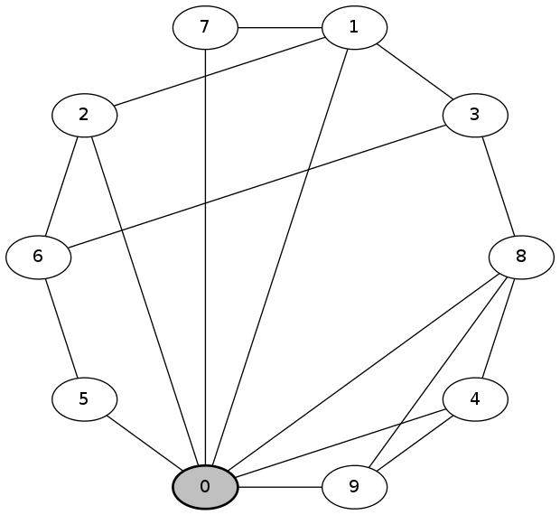
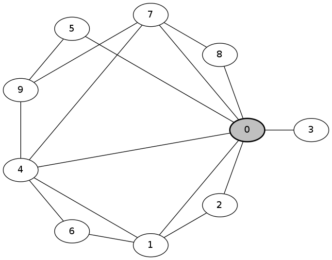
SMC suffer from the fact that high confidence required by an answer may demand a large number of simulation runs, each of which may itself be time consuming. As an example, the first hypothesis test shown later in this section can generate between 14,000 and 2,390,000 runs if the parameters α, β, δ range between 0.01 and 0.001. A possible way to leverage this problem is to use several computers working in parallel using a master/slaves architecture: one or more slave processes register their ability to generate simulation with a single master process that is used to collect those simulations and peform the statistical test. When working with an estimation algorithm, this collection is trivially performed as the number of simulations to perform is known in advance and can be equally distributed between the slaves.
When working with sequential algorithms, the situation gets more complicated. Indeed, we need to avoid introducing bias when collecting the results produced by the slave computers. We make a model of the simple case where the master collects results arbitrarily from the slaves to pinpoint the bias problem.
Distributed hypothesis testing algorithm model/query files.
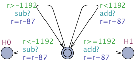 |
| Master node. |
| |
 |
| Slave node. |
Comparison with PVesta
We compare the distributed Uppaal SMC implementation with the PVesta toolset. In doing so we consider the cyclic polling server example (distributed with PVesta) where a job server polls a job stations for a job, serves the station if there is a job or moves on to the next station. The model is parameterised by the number of job stations.
We created a Uppaal model and query and used the model provided by the PVesta toolset for the comparison. We used models with 900 stations for the comparison and repeated the experiment ten times. The results in the table are averages of these ten runs.
Uppaal succeeded in verifying the model with only one processing node in less than one 4 seconds thus we write ≤ 4 for all cases - otherwise we would be measuring the time for setting up the processing nodes. It is well-known that the sequential probability ratio test used by UPPAAL in many cases is faster than the single sampling plan approach, used by PVesta, thus unsurprisingly Uppaal is faster than PVesta regarding hypothesis testing. An indication as to why can be seen in the table where Uppaal uses remarkably fewer samples than Pvesta.
The single sampling plan approach resembles the approach for probability estimation used in distributed UPPAAL SMC. We estimate the probability that query holds with confidence 99.1. In this setting UPPAAL generates 18448 samples - which is more samples than used by PVesta. We notice Uppaal generates the 18448 samples faster than Pvesta. We also notice that both toolsets scale almost linearly in the number of processing nodes.
For Uppaal to be slower than PVesta we had to scale the model to use 9000 stations - and even then only estimation was slower.
Model file.
Estimation query.
Hypothesis testing query.
| |||||||||||||||||||||||||||||||||||||||||||||||||||
| Performance comparison between PVesta and UPPAAL. Time is in seconds. | |||||||||||||||||||||||||||||||||||||||||||||||||||
Control-SMC
Control-SMC is a new extension of UPPAAL-TIGA. It automatically synthesizes a strategy of a timed game with respect to a control objective, keeps the strategy in memory, then verifies and evaluates the strategy. It combines the engines from UPPAAL-TIGA, UPPAAL and UPPAAL-SMC. At present, Control-SMC is implemented as a module inside the command line version of UPPAAl-TIGA, and is enabled by the option -X. In the long term, this functionality will be available in a unified version of UPPAAL and UPPAAL-TIGA.
We can use UPPAAL-TIGA (GUI) for modelling and run Control-SMC on the command line for model checking and statistical model checking. Control-SMC is a command line tool verifytga on Windows/Mac/Linux.
Usage:
- Use
verifytga -w0to get the strategy for a timed game model and a control objective. - Use
verifytga -Xto enable Control-SMC. Note the query file should have the control query on the first line and MC and SMC queries on the following lines. - Use
verifytga -X -E εto set probability uncertainty (a.k.a. precision) factor ε on checking the SMC queries. Note -E is only selectable when -X is present.
Here are one running example and two case studies to demonstrate the usefulness of Control-SMC.
| Running Example | Model | Query |
| Case Study 1: Jobshop | Model | Query |
| Case Study 2: Train-Gate | Model | Query |
There is another way to verify and evaluate the strategy. First, translate the strategy into a controller timed automaton. Second, build a closed system using the controller and the timed game model. Third, check the MC and SMC queries of the closed system by UPPAAL and UPPAAL-SMC. We also provide models, query files, translated controller for the running example and the case studies mentioned above.
| Running Example | Game Model | MC Model | SMC Model |
| Control Query | MC Query | SMC Query | |
| Case Study 1: Jobshop | Game Model | MC Model | SMC Model |
| Control Query | MC Query | SMC Query | |
| Case Study 2: Train-Gate | Game Model | MC Model | SMC Model |
| Control Query | MC Query | SMC Query |
 |
| Running Example. |
| |
 |
| Case Study 1: Jobshop. |
| |
 |
| Case Study 2: Train-Gate. |