Optimizing Control Strategy using Statistical Model Checking
This page contains technical information required to replicate the controller optimization experiment as described in the following publication:
Alexandre David, Kim Guldstrand Larsen, Marius Mikučionis, Axel Legay and Dehui Du: Optmizing Control Strategy using Statistical Model Checking. To appear in the proceedings of NASA Formal Methods 2013.
All the files can be downloaded in one archive: ANOVA-SMC-data.zip.
The following map shows an overview of entire experiment setup with links to individual steps.

Model
This experiment is a continuation of a previous study described in the following publication:
Alexandre David, DeHui Du, Kim G. Larsen, Marius Mikučionis, Arne Skou: An evaluation framework for energy aware buildings using statistical model checking. Science China Information Sciences December 2012, Volume 55, Issue 12, pp 2694-2707 [bib]
In this experiment with fix the user and environment models and vary the controller parameter values in order to find the optimal ones. File pareto.xml contains the Uppaal model of an energy aware building with two levels of control. The local (room) level controller is parameterized with Ton temperature threshold when to turn on the heater, and the global controller is parameterized with Tget temperature threshold to denote that a heater is needed in a particular room. The building layout is shown in the figure below.

Query
The goal here is to instruct the tool to record the final values of the parameter and cost variables. File discomfort.q contains the Uppaal query:
simulate 1200 [<=2*day] { tday[1].Ton, tday[1].Tget, discomfort, Global.energy } : 1 : false
The query instructs to perform 1200 simulations of up to 2 days of model time and record the trajectories of Ton, Tget, discomfort and energy variables.
Without :1:false part the query would generate the trajectories requiring a lot of extra memory just to keep them, but we are interested only in the values of the final state, thus we would like to get rid of this overhead. This extra tail instructs the tool to keep generating the runs until 1 run is found to satisfy false property, however none of the runs can satisfy false and thus the tool discards all the trajectory data.
The next step shows how the last state variables values are preserved.
Data Generation
The following command is used launch Uppaal verifier at the command line to generate stochastic runs and gather the data:
UPPAAL_DUMP_STATE=1 verifyta parretto.xml discomfort.q > /dev/null
The environment variable UPPAAL_DUMP_STATE=1 setting turns on the logging of the last state into simulation_tail.log file. The log contains the final values of time, parameters (temperature threshold) and cost variables (discomfort and energy) as requested by the query.
The parameter and cost values can be extracted by filtering the corresponding columns:
gawk '{ print $2" "$4" "$6" "$8 }' simulation_tail.log > data.log
The data is saved into data.log file.
Below is a scatter plot of differently colored parameter configurations by discomfort time and energy cost.
Notice that it is hard to distinguish the colored clusters and choose an optimal one, hence a statistical analysis using ANOVA method is performed.
Balancing
Before ANOVA can be performed, the data has to be balanced in a sense that every parameter configuration should have the same amount of records. File balance.cpp contains a small C++ program gathering the records from standard input stream and outputting the balanced records into output stream when entire level across configurations is filled. When the input stream is finished the unbalanced data is discarded. The program is compiled using GNU Compiler:
g++ -O3 balance.cpp -o balance
Then the simulation data can be balanced using the following command:
./balance < data.log > dataF.dat
Notice that commands can be combined into single pipe while verifyta is still generating data in the background:
gawk '{ print $2" "$4" "$6" "$8 }' simulation_tail.log | ./balance > dataF.dat
The result is saved into dataF.dat file.
ANOVA
File anovaF.R contains an R project script performing the ANOVA. The script uses loaddata.R script to load the data from dataF.dat, then it checks that the data is really balanced and performs ANOVA. The script is launched by the following command:
R --quiet --no-save < anovaF.R
Below is an example output:
Analysis of Variance Table

Response: discomfort
            Df Sum Sq Mean Sq   F value    Pr(>F)
Ton          1 372627  372627 6638.5603 < 2.2e-16 ***
Tget         1   1006    1006   17.9244 2.324e-05 ***
Ton:Tget     1     36      36    0.6485    0.4207
Residuals 8130 456342      56
---
Signif. codes:  0 ‘***’ 0.001 ‘**’ 0.01 ‘*’ 0.05 ‘.’ 0.1 ‘ ’ 1
> coef(d_aov) # compute linear model coefficients
(Intercept)         Ton        Tget    Ton:Tget
91.20298401 -3.70193864 -0.49359600  0.01672352
>
> e_aov <- aov(energy ~ Ton * Tget, data=raw) ; anova(e_aov)
Analysis of Variance Table

Response: energy
            Df  Sum Sq Mean Sq   F value Pr(>F)
Ton          1  105522  105522  163.2509 <2e-16 ***
Tget         1  712025  712025 1101.5637 <2e-16 ***
Ton:Tget     1    1084    1084    1.6774 0.1953
Residuals 8130 5255043     646
---
Signif. codes:  0 ‘***’ 0.001 ‘**’ 0.01 ‘*’ 0.05 ‘.’ 0.1 ‘ ’ 1
> coef(e_aov)
 (Intercept)          Ton         Tget     Ton:Tget
131.65442935   0.06667493   2.94383693   0.09127479
One may stop the data generation and cancel verifyta process when the chosen factors reach required significance (for example the factor row contains three stars ***) and move on to the next step of estimating the actual means.
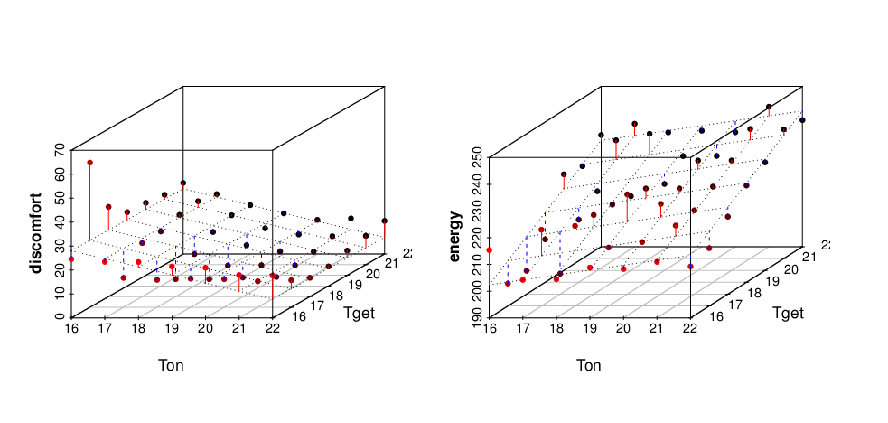
ANOVA method also computes the coefficients of a linear model and thus the data can be approximated by a plane. File linearmodel.R contains R-project script generating 3D plot of a linear fitted models shown below:

Computing Means
File means.F contains an R-project script which reads the data from file dataF.dat, computes the mean cost with standard deviation for each parameter configuration and saves the data into means.dat.
Pareto Frontier
Pareto frontier is computed by finding the cost-dominating configurations. File dominators.cpp contains C++ program used to compute the dominating parameter configurations. File dominators-means.cpp contains C++ program used to compute the parameter configurations dominating by mean cost. The programs are compiled using the following commands:
g++ -O3 dominators.cpp -o dominators
g++ -O3 dominators-means.cpp -o dominators-means
Then Pareto frontiers are computed by executing the following command:
gawk '{ print $1" "$2" "$3" "$4 }' dataF.dat | ./dominators > pareto.dat
./dominators-means < means.dat > means-pareto.dat
The means with error bars and Pareto frontiers are then plotted into means.eps image file using GNU Plot script meansF.plot:
gnuplot meansF.plot
Figure below shows an example result (meansSVG.plot) where Pareto optimal configurations are marked by rectangles.
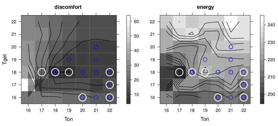
Alternatively the configurations can be visualized in level maps where the cost is encoded by a color shade. File paretoF.R contains R-project script producing level-plots discomfort-levels-b.eps and energy-levels-b.eps where Pareto optimal configurations are marks by white circles.
An example result is shown below:
