CORA Case Studies and Examples

• Vehicle Routing Problem with Time Windows
• Aircraft Landing Problem
• Energy Optimal Task Graph Scheduling

Vehicle Routing Problem with Time Windows

The vehicle routing problem with time windows (VRPTW) is a generalization of the travelling salesman problem with multiple salesmen. Consider a business located at (0,0) in a two-dimensional coordinate system. The business produces some goods and ships it to a number of dispersed customers in the coordinate system. Each customer has a specific demand and must be served within a given time window. Available to the business is a fleet of vehicles with limited capacity, now, the problem is to assign routes to each vehicle such that each customer demand is met within the designated time windows and the vehicle returns to the business. Several objective functions can be used for optimization in this scenario, e.g. the total length of the routes, the total time taken to execute the routes, etc.

Input

We are given a number of customers C_i=(x_i,y_i,d_i,e_i,l_i) where (x_i,y_i)) is the location of the customer, d_i is the demand, and [e_i,l_i] is the time window. Furthermore, we a given a number, m, of vehicles with capacity c.

Problem

Assign to each vehicle a route such that:

• The objective function is minimized.
• The total demand of a route does not exceed c.
• Each customer on the route will be visited in the interval [e_i,l_i].

The particular objective function used in the example is the sum of a ⋅ sum(distance) + b ⋅ end_time + c ⋅ (max(0, sum(demand)-K)) for every route, where a,b,c are constants and K is some percentage of the capacity.

Download

The UPPAAL model and specification can be downloaded.

Aircraft Landing Problem

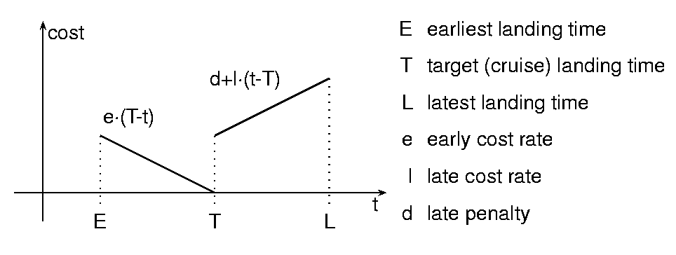
The aircraft landing problem (ALP) was first provided in [BKS00] solved using mixed integer linear programming (MILP). The problem consists of a number of aircrafts that need to land on limited number of runways. Each aircraft has a preferred target landing time, corresponding to arriving at the runway with cruise speed and landing immediately. However, the aircraft can speed up and land earlier or stay longer in the air and land later if necessary. Due to extra gas used in accelerating, landing earlier has an added cost which grows linearly until some fixed earliest landing time. Late landings have an immediate constant penalty for landing late and a cost growing linearly with the amount of gas used for staying in the air until all latest possible (controlled) landing time. The cost function for a single aircraft is given in the figure below.

Furthermore, aircrafts cannot land back to back on the same runway due to wake turbulence. Thus, there are certain minimum constraints on the separation delay between aircrafts of different types, e.g. a Boeing 747 can handle (and generates) more turbulence than a Hawker 700.

Now, the problem is to assign landing times and runways to all aircrafts while respecting individual timing constraints for the aircrafts and the wake turbulence constraints.

Input

We are given a number aircrafts with A_i=(E_i,T_i,L_i,e_i,l_i,d_i,k_i) where k_i is the kind of aircraft and the rest of the parameters are as given in the figure above. The parameters for each aircraft define a function:

as depicted in the figure above. Furthermore, separation function sep(a,b), which gives the required separation between two aircrafts of types a and b landing on the same runway. Finally, we are given a number, R, of runways.

Problem

Assign to each aircraft A_i a landing time E_i ≤ t_i ≤ L_i and a runway 1 ≤ r_i ≤ R such that

• ∑_i C_i(t_i) is minimal
• sep(k_i,k_j) ≤ k_i-k_j whenever i ≠ j, t_i ≥ t_j, and r_i = r_j.

Download

The UPPAAL model and specification can be downloaded.

Energy Optimal Task Graph Scheduling

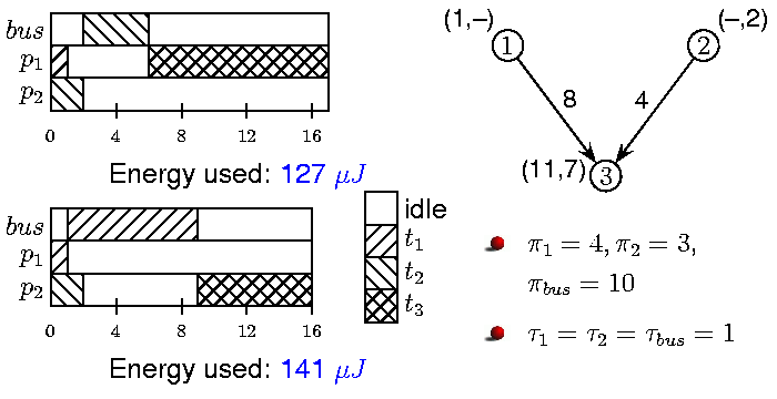
Energy-optimal task graph scheduling (ETGS) is the problem of scheduling a number of interdependent tasks onto a number heterogeneous processors that communicate through a single bus while minimizing the overall energy requirement and meeting an overall deadline. The interdependencies state that a task cannot execute until the results of all predecessors in the graph have been computed. Moreover, the results should be available in the sense that either each of the predecessors have been computed on the same processor, or on a different processor and the result has been broadcasted on the bus. An example task graph with three tasks is depicted in the figure below. The task t₃ cannot start executing until the results of both tasks t₁ and t₂ are available. The available resources are two processors, p₁ and p₂, and a single bus with energy consumptions π₁=4, π₂=3, and π_bus=10 per time unit when operating and 1 when idle. For real applications energy consumption is, usually, measured in mW and execution times in ms. The nodes in the figure are annotated with their execution times on the processors, that is, t₁ can only execute on p₁, t₂ only on p₂, and t₃ can execute on both p₁ and p₂.

The energy-optimal schedule is achieved by letting t₁ and t₂ execute on p₁ and p₂, respectively, broadcast the result of t₂ on the bus, and execute t₃ on p₁, which consumes the total of 127 energy units. On the other hand, broadcasting the result of t₁ on the bus and executing t₃ on p₂ requires 141 energy units. Both schedules are depicted as Gantt charts in the figure.

Input

The ETGS problem is given as a 8-tuple (T,P,<,δ,π,τ,κ,D) where T={t₁,…,t_n} is a the set of tasks, P={p₁,…,p_k} is the set of processors (or machines), < is an irreflexive preorder on T giving the precedence constraints, δ = {δ₁₁,δ_n1,δ₁₂,…,δ_nk} where each δ_ij∈ N ∪ {∞}, N is the set of natural numbers, gives the execution time of task t_i on processor p_j, π = {π_bus,π₁,…,π_k} gives the energy consumption of the bus and processor while operating, τ = {τ_bus,τ₁,…,τ_k} gives the energy consumption of the bus and processor while idle, κ = {κ₁,…,κ_n} gives the communication time for sending tasks over the bus, and D is the deadline.

Problem

Assign to each task, t_i, a triple (a_i,b_i,c_i) stating that at time a_i, task t_i should start executing on processor b_i and the result should be broadcasted on the bus at time c_i. This assignment should minimizes the total energy consumption while respecting the precedence constraints and never letting the bus or processors be utilized by more than one task at any time.